(Solved): quantum mechanics of the eigenfunctions \( \psi_{ ...

quantum mechanics

??????????????

of the eigenfunctions \( \psi_{n 1} \). 4.7 The Isotropic Harmonic Oscillator. In Section \( 2.9 \) we analyzed the three-dimensional harmonic os cillator using cartesian coordinates. However, the use of cartesian coordinates, although verysimple, is not optimal for obtaining information about the angular momentum and sertain other features of the isotropic oscillator. Since the potential energy of an isotropic harmonic oscillator is \( V=\frac{1}{R} k r^{2} \), corresponding to a central force problem, it is desirable to employ spherical coordinates. Inserting the potential energy into the radial equation \( (4,4-4) \) we find \[ \frac{\mathrm{d}^{2} u}{\mathrm{~d} r^{2}}+\left[\frac{2 \mathrm{k}^{2}}{k^{\varepsilon}}\left(E-\frac{1}{2} k r^{2}\right)-\frac{2(1+1)}{r^{3}}\right] \mathrm{u}=0 . \] The solution of \( \{4,7-1\} \) gives the allowed values of the energy for each angular momentum state, If we write \( r=a p \) with \( a=\sqrt{f} \) and reduces to \[ \mathrm{d}^{2} u / \mathrm{d} r^{2}+\left[C-p^{2}-1(1+1) / p^{2}\right] u=0 \] The asymptotic form of this equation for \( r \rightarrow \infty \) is \( \mathrm{d}^{2} u / d \rho^{2}-\rho^{2} u=0 \) ch admits of a solution cussion in Section \( 4.4 \) regh \( u(\rho)=\rho^{1+1} e^{-\rho^{2}} / e_{f(\rho)} d \) \( (4.7-2) \) which admits of a solution \( \left(\mu(\rho) \sim e^{-\rho} / 2\right) \) In accordance \( \quad(4,7-3) \) discussion in Section 4.4 regarding the behavior of the radial wave function when \( m \sim 0 \), one should write the radial wave function as 5 Substituting this form into \( (4,7-2) \) we arrive at the differential equation for \( f(\rho) \), \[ \rho\left(\mathrm{d}^{3} f / \mathrm{d} \rho^{2}\right)+2\left(1+1-\rho^{2}\right) \mathrm{d} f / \mathrm{dp}-(21+3-C) \rho f=0 . \] Making a new change of variable \( \mathrm{g}=\rho^{3} \), one 18 led to the equation \( 5 \mathrm{~d}^{2} f / \mathrm{d} \xi^{n}+\left(1+\frac{a}{2}-\xi\right) \mathrm{d} f / \mathrm{d} \xi-\frac{1}{4}(21+3-C) f=0 \). But this is of the form of the well-known differential equation \[ 5 \vec{F} \|+(b-5) F(-a F=0, \] \( (4.7-5) \) the solution of which is the confluent hypergeometric series \( F(a, b, b)=\sum \frac{\Gamma(a+8) \Gamma(b) g^{n}}{\Gamma(a) \Gamma(b+s) \Gamma(\varepsilon+1)}=1+\frac{a g}{b}+\frac{a(a+1) g^{z}}{b(b+1) 2 !}+\ldots(4,7-6) \) Thus \( f\left(p^{2}\right)=F\left[\frac{1}{4}(21+3-C), 1+\frac{3}{2}, p^{2}\right] \) and \( (4,7-4) \) becomes \( u(\rho)=p^{1+1} e^{-\rho^{2} / 2} F\left[\frac{1}{4}(21+3-C), l+\frac{3}{2}, p^{2}\right] \). \( (4,7-7) \) For large \( s, F \) behaves as \( e^{5} \) or \( e^{\rho^{2}} \), as it can be easily verified from \( (4,7-6) \), so that \( \left.u(0) \rightarrow D^{1+1} e^{\rho}\right)^{\prime} \), which is not normalizable. 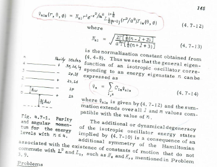Therefore instead of a series, \( F \) must be a polynomial terminating at some specific value of \( \varepsilon \), a fact that requires that \( a+8=0 \) or \( C=2 l+3+48 \). Note that the degree of the polynomial in \( p \) is \( 2 a \) (an even number). It follows from the definition of \( C \) that the energy of a stationary state is \[ E=\left(28+1+\frac{3}{2}\right) \hbar w, \] A comparison of this result with \( (2.9-8) \) shows that \( n \) and 7 are related by \( n=2 s+1 \), implying that \( n \) and \( I \) are simultaneously either even or odd. Thus each energy state \( n \) is associated with several orbital angular momentum states \( l \) according to \[ 1=n-28=n, n-2, \ldots, \text { (1 or } 0 \text { ). } \] If we look back at the discussion of the three-dimensional os cillator in Section \( 3.9 \), we note that the possible values of \( m\left(=r_{4}-r_{-}\right) \) listed in Table 3.9-1 are precisely those required by the values of \( I \) listed in (4,7-9). Furthermore since each \( I \) state has a geometrical degeneracy of \( 2 l+1 \), we see that the total degeneracy of the energy state is \[ \left.q=\sum_{\substack{1 \\ \text { even or odd }}}(2)+1\right)=\frac{1}{2}(n+1)(n+2) \] a result in agreement with \( (2.9-9) \). The different states of the oscillator are designated by a letter, s, p, d,... corresponding to the angular momentum, and with a number \( v=\frac{1}{2}(n-1)+1 \) which indicates the order of appearance of the angular momentum as the energy increases, It can be easily verified that \( v \) is the number of roots of \( R_{91}(r) \), excluding the origin but including \( r=\infty \). Figure 4, 7-1 illustrates the properties of the first few states. We now return to the problem of constructing the appropriate energy eigenfunctions. From the identification of \( n \) we note that \( C=2 n+3 \). Inserting this value into \( (4,7-7) \) we can rewrite it as \[ u_{\mathrm{n} 1}(p)=p^{1+1} e^{-p^{3} h_{F}}\left[\frac{1}{2}(1-n), 1+\frac{p}{2}, p^{3}\right] \text {, } \] or invoking the definition of the Laguerre polynomial \( { }^{(3)} \) in terms of the hypergeometric function, \( L_{p}^{q}(x)=F(-p, q+1, x) \) given in Appendix C. 4 The complete oscillator eigenfunctions are, therefore, \( \phi_{\mathrm{nta}}\left(r^{\prime}, \theta, \phi\right)=N_{\mathrm{ad}} \Gamma^{1} e^{-r^{2} / x_{a}^{2}} \sum_{\frac{1}{2}(1-1)}^{1+\frac{1}{2}}\left(r^{2} / a^{2}\right) Y_{\mathrm{l}}(\theta, \phi) \) where \( (4,7-12) \) \[ N_{n 1}=\sqrt{\frac{2 T\left[\frac{1}{2}(n-1+2)\right]}{a^{2} T\left[\frac{1}{2}(n+1+3)\right]}} \] \( (4.7-13) \) is the normalization constant obtained from \( (4.4-8) \). Thus we seethat the general eigenRurity scates function of an isotropic oscillator corre\( +3 g, 2 d, l g \) sponding to an energy eigenstate \( n \) canbe \( \begin{array}{lll}- & 2_{p}, 1 f & \text { expresased as } \\ + & 2 s, 1 d & \\ - & 2 p & \psi_{n}=\sum_{d, \pi} C_{L_{n} \phi_{n \pi}} \\ + & 1 s & \end{array} \)