(Solved): MATLAB - QUESTION 4 ONLY For example, consider the IVP problem \[ \frac{d y}{d t}=f(t, y), y(0) ...

MATLAB - QUESTION 4 ONLY

For example, consider the IVP problem \[ \frac{d y}{d t}=f(t, y), y(0)=1,0 \leq t \leq 2 ? \] where \( f(t, y)=1-e^{-4 t}-2 y \). We can define \( f(t, y) \) as an anonymous function: \[ f=@(t, y) 1-\exp (-4 * t)-2 * y ; \] Then we solve the IVP with the command ode45: \[ [t, y]=\operatorname{ode45}\left(f,\left[\begin{array}{ll} 0 & 2 \end{array}\right], 1\right) ; \] Finally we plot the solution: How would you change these commands to solve the IVP for the same ODE but with the condition \( y(1)=1 \) on the interval \( 1 \leq t \leq 3 \) ? Try it and re-run this section to see the result. 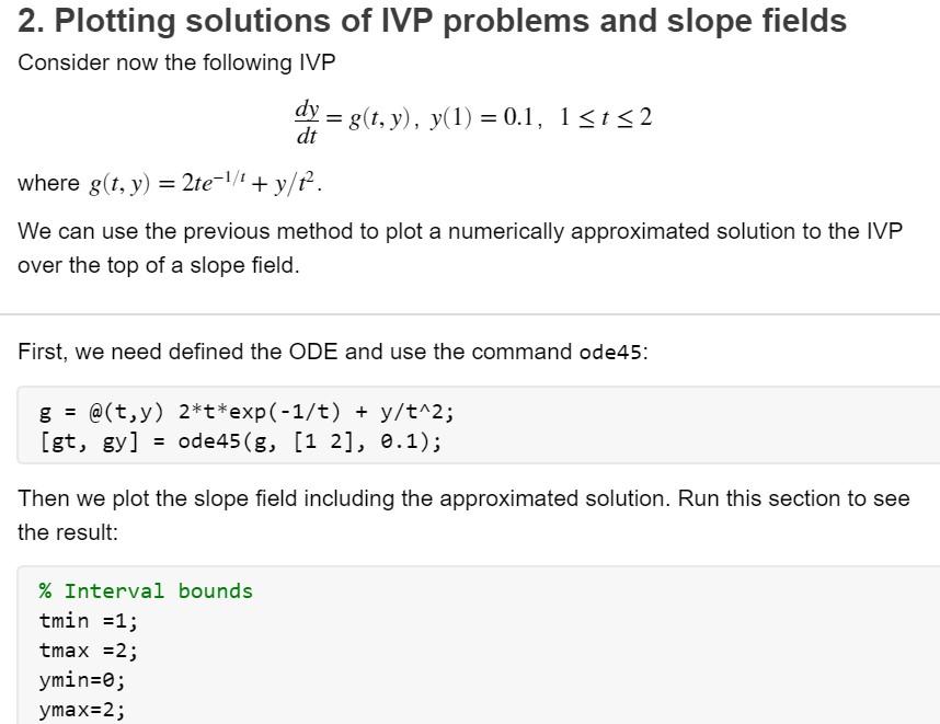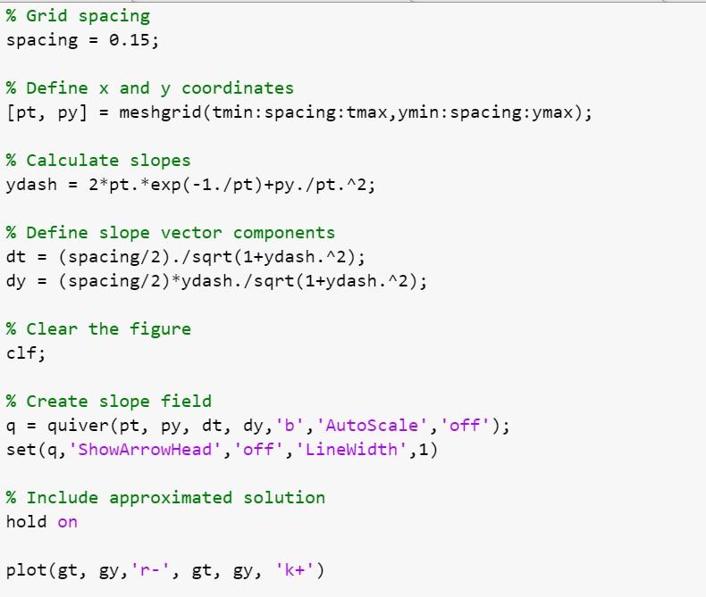2. Plotting solutions of IVP problems and slope fields Consider now the following IVP \[ \frac{d y}{d t}=g(t, y), y(1)=0.1,1 \leq t \leq 2 \] where \( g(t, y)=2 t e^{-1 / t}+y / t^{2} \) We can use the previous method to plot a numerically approximated solution to the IVP over the top of a slope field. First, we need defined the ODE and use the command ode45: \[ \begin{array}{l} g=@(t, y) 2 * t * \exp (-1 / t)+y / t^{\wedge} 2 ; \\ {[g t, g y]=\operatorname{ode45}\left(g,\left[\begin{array}{ll} 1 & 2 \end{array}\right], 0.1\right) ;} \end{array} \] Then we plot the slope field including the approximated solution. Run this section to see the result: \( \% \) Interval bounds tmin \( =1 ; \) tmax \( =2 ; \) ymin=0; ymax \( =2 ; \) hold off \% Set axis and labels axis([tmin tmax ymin ymax]) xlabel(' \( x \) ') ylabel(' \( y \) ') Note: In the previous code we used the command set( ) to set graphics object properties. For more details see: Set Graphics Object. 3. Systems of differential equations Anonymous function can also be used to define systems of ODEs. The easiest way to think of this is that the function will take a vector of inputs \( Y \) and puts the inputs into a vector of equations. For example, a second order ODE of the form \[ z^{\prime \prime}+z^{\prime}-z=\cos (t) \] can be expressed as the coupled system of equations. Let \( z^{\prime}=y \). Then we have that \( z^{\prime \prime}=y^{\prime} \). 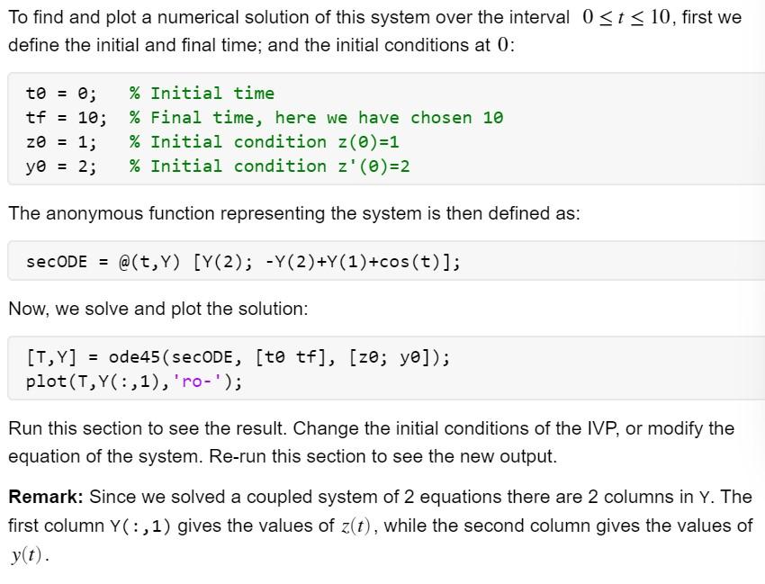If we substitute in equation (1) we obtain the system: \[ \begin{array}{l} z^{\prime}=y \\ y^{\prime}=-y+z+\cos (t) \end{array} \] Define the vector \( Y \) as \[ Y=\left(\begin{array}{l} z \\ y \end{array}\right) \] The derivative of \( Y \) is a vector whose entries correspond to the coupled equations: \[ Y^{\prime}=\left(\begin{array}{l} z^{\prime} \\ y^{\prime} \end{array}\right)=\left(\begin{array}{c} y \\ -y+z+\cos (t) \end{array}\right) \] Now we have two first order equations that we can store as a vector of anonymous functions with vector input \( Y \). We do this by writting: \[ \sec O D E=@(t, Y)[Y(2) ;-Y(2)+Y(1)+\cos (t)] ; \] 3.1 Numerical solution of systems of ODEs Now consider the IVP \[ z^{\prime \prime}+z^{\prime}-z=\cos (t), z(0)=1, z^{\prime}(0)=2,0 \leq t \leq 10 . \] which can be re-written as \[ \begin{array}{l} z^{\prime}=y \\ y^{\prime}=-y+z+\cos (t), z(0)=1, z^{\prime}(0)=2,0 \leq t \leq 10 . \end{array} \] To find and plot a numerical solution of this system over the interval \( 0 \leq t \leq 10 \), first we define the initial and final time; and the initial conditions at 0 : The anonymous function representing the system is then defined as: \[ \operatorname{secODE}=@(t, Y)[Y(2) ;-Y(2)+Y(1)+\cos (t)] \] Now, we solve and plot the solution: \[ \begin{array}{l} {[T, Y]=\operatorname{ode} 45(\operatorname{secODE},[t \theta t f],[z \theta ; y \theta]) ;} \\ p \operatorname{lot}(T, Y(:, 1) \text {, 'ro-'); } \end{array} \] Run this section to see the result. Change the initial conditions of the IVP, or modify the equation of the system. Re-run this section to see the new output. Remark: Since we solved a coupled system of 2 equations there are 2 columns in \( Y \). The first column \( Y(:, 1) \) gives the values of \( z(t) \), while the second column gives the values of \( y(t) \). 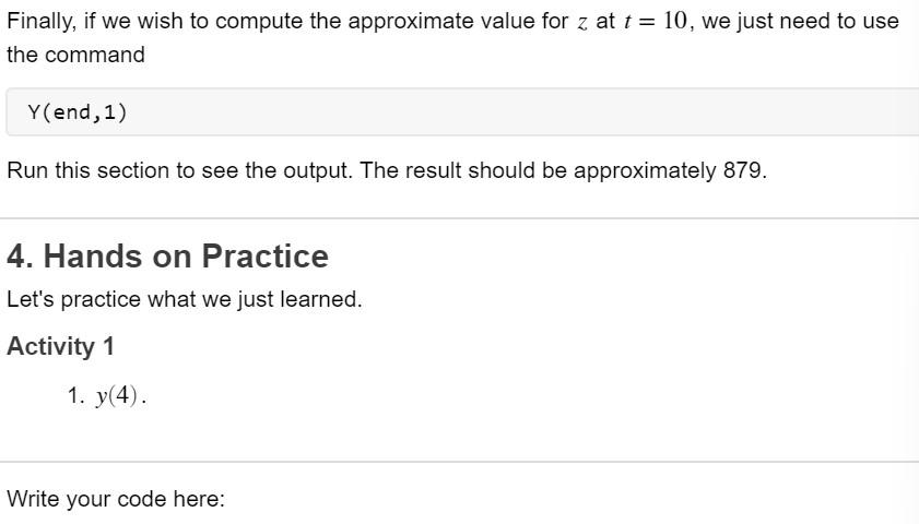Finally, if we wish to compute the approximate value for \( z \) at \( t=10 \), we just need to use the command \( Y( \) end, 1\( ) \) Run this section to see the output. The result should be approximately 879 . 4. Hands on Practice Let's practice what we just learned. Activity 1 1. \( y(4) \). Write your code here: