(Solved): Grader - Instructions Excel 2022 Project Exp22_Excel_Ch07_ML2_Employees Project Description: You ...

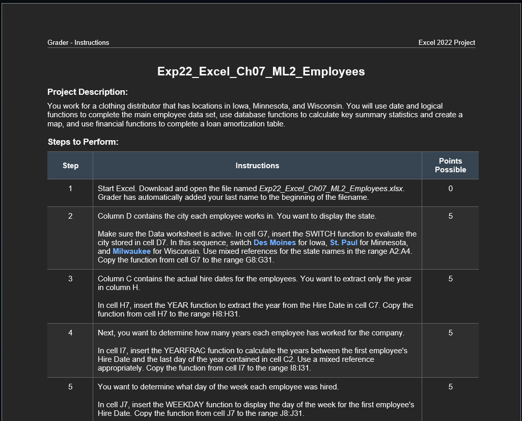
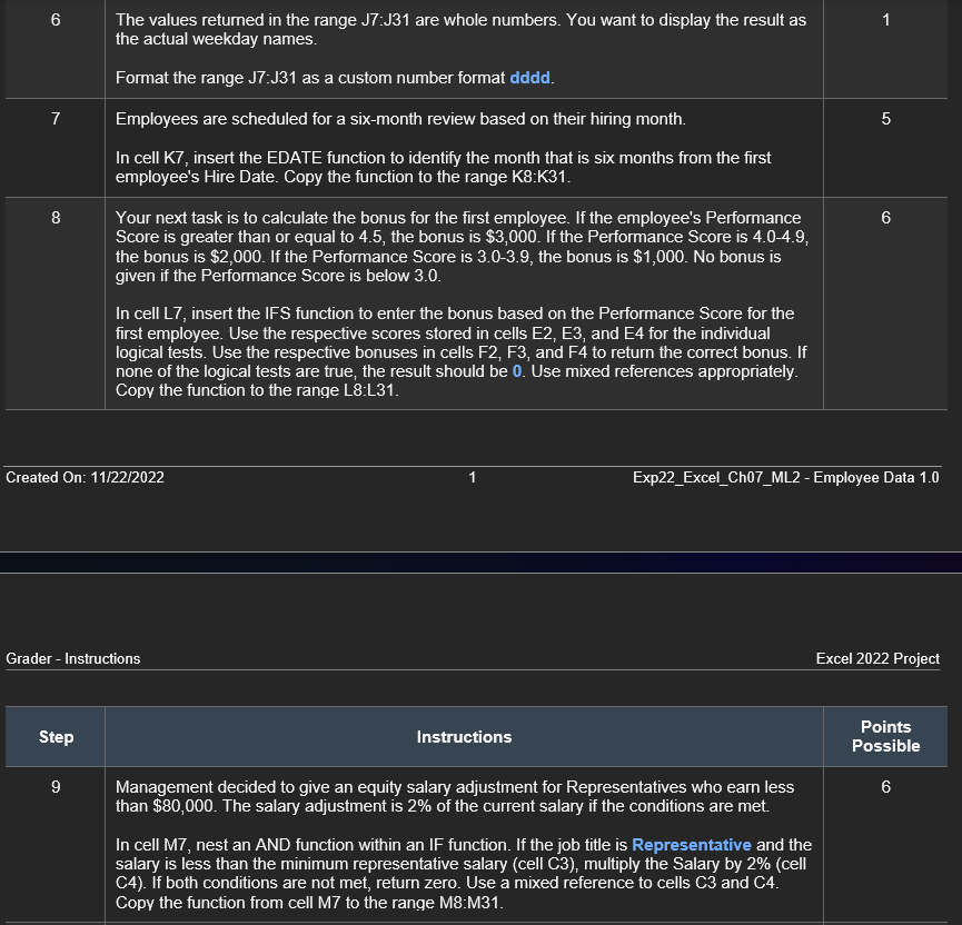
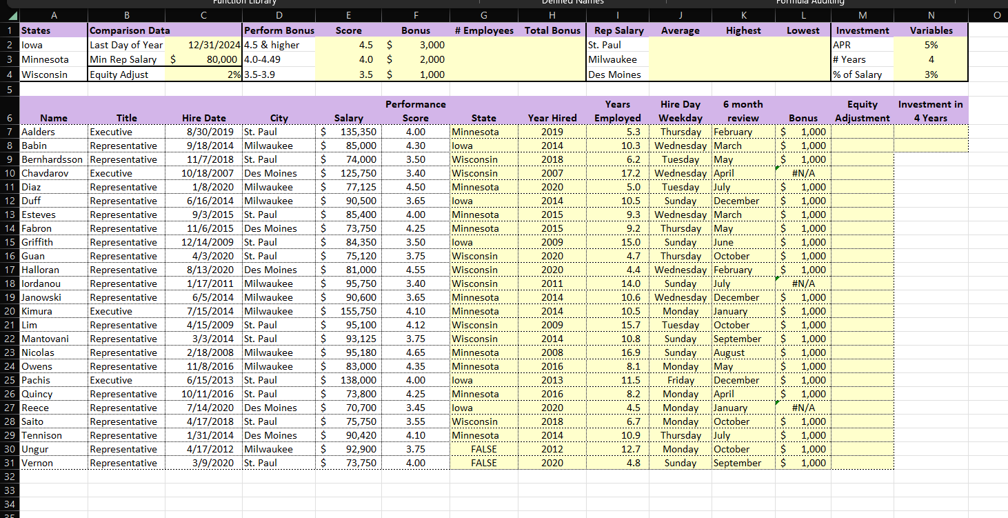
Grader - Instructions Excel 2022 Project Exp22_Excel_Ch07_ML2_Employees Project Description: You work for a clothing distributor that has locations in lowa, Minnesota, and Wisconsin. You will use date and logical functions to complete the main employee data set, use database functions to calculate key summary statistics and create a map, and use financial functions to complete a loan amortization table. Steps to Perform: \begin{tabular}{c|l|c} \hline Step & \multicolumn{1}{|c|}{ Instructions } & \multicolumn{1}{c}{ Points } \\ \hline 1 & Start Excel. Download and open the file named Exp22_Excel_ChO7_ML2_Employees.xlsx. Grader has automatically added your last name to the beginning of the filename. \\ \hline 2 & Column D contains the city each employee works in. You want to display the state. Make sure the Data worksheet is active. In cell G7, insert the SWITCH function to evaluate the city stored in cell D7. In this sequence, switch Des Moines for lowa, St. Paul for Minnesota, and Milwaukee for Wisconsin. Use mixed references for the state names in the range A2:A4. Copy the function from cell G7 to the range G8:G31. & 5 \\ \hline 3 & Column C contains the actual hire dates for the employees. You want to extract only the year in column H. & 5 \\ \hline In cell H7, insert the YEAR function to extract the year from the Hire Date in cell C7. Copy the function from cell H7 to the range H8:H31. & 5 \\ \hline 4 & Next, you want to determine how many years each employee has worked for the company. In cell I7, insert the YEARFRAC function to calculate the years between the first employee's Hire Date and the last day of the year contained in cell C2. Use a mixed reference appropriately. Copy the function from cell I7 to the range I8:I31. & 5 \\ \hline 5 & You want to determine what day of the week each employee was hired. In cell J7, insert the WEEKDAY function to display the day of the week for the first employee's Hire Date. Copy the function from cell J7 to the range J8:J31. 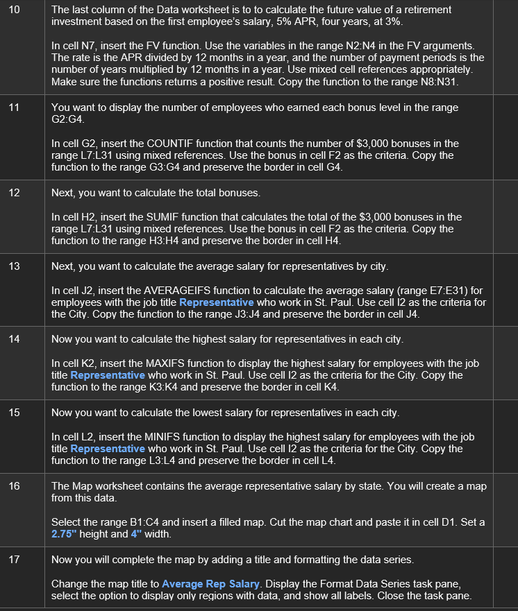\\ \hline \end{tabular} Grader - Instructions The last column of the Data worksheet is to to calculate the future value of a retirement investment based on the first employee's salary, \( 5 \% \) APR, four years, at \( 3 \% \). In cell N7, insert the FV function. Use the variables in the range N2:N4 in the FV arguments. The rate is the APR divided by 12 months in a year, and the number of payment periods is the number of years multiplied by 12 months in a year. Use mixed cell references appropriately. Make sure the functions returns a positive result. Copy the function to the range N8:N31. You want to display the number of employees who earned each bonus level in the range G2:G4. In cell G2, insert the COUNTIF function that counts the number of \( \$ 3,000 \) bonuses in the range L7:L31 using mixed references. Use the bonus in cell F2 as the criteria. Copy the function to the range G3:G4 and preserve the border in cell G4. Next, you want to calculate the total bonuses. In cell \( \mathrm{H} 2 \), insert the SUMIF function that calculates the total of the \( \$ 3,000 \) bonuses in the range L7:L31 using mixed references. Use the bonus in cell F2 as the criteria. Copy the function to the range \( \mathrm{H} 3: \mathrm{H} 4 \) and preserve the border in cell \( \mathrm{H} 4 \). Next, you want to calculate the average salary for representatives by city. In cell J2, insert the AVERAGEIFS function to calculate the average salary (range E7:E31) for employees with the job title Representative who work in St. Paul. Use cell 12 as the criteria for the City. Copy the function to the range J3:J4 and preserve the border in cell J4. Now you want to calculate the highest salary for representatives in each city. In cell K2, insert the MAXIFS function to display the highest salary for employees with the job title Representative who work in St. Paul. Use cell I 2 as the criteria for the City. Copy the function to the range K3:K4 and preserve the border in cell K4. Now you want to calculate the lowest salary for representatives in each city. In cell L2, insert the MINIFS function to display the highest salary for employees with the job title Representative who work in St. Paul. Use cell I2 as the criteria for the City. Copy the function to the range L3:L4 and preserve the border in cell L4. The Map worksheet contains the average representative salary by state. You will create a map from this data. Select the range B1:C4 and insert a filled map. Cut the map chart and paste it in cell D1. Set a \( 2.75^{\prime \prime} \) height and \( 4^{\text {" }} \) width. Now you will complete the map by adding a title and formatting the data series. Change the map title to Average Rep Salary. Display the Format Data Series task pane, select the option to display only regions with data, and show all labels. Close the task pane. 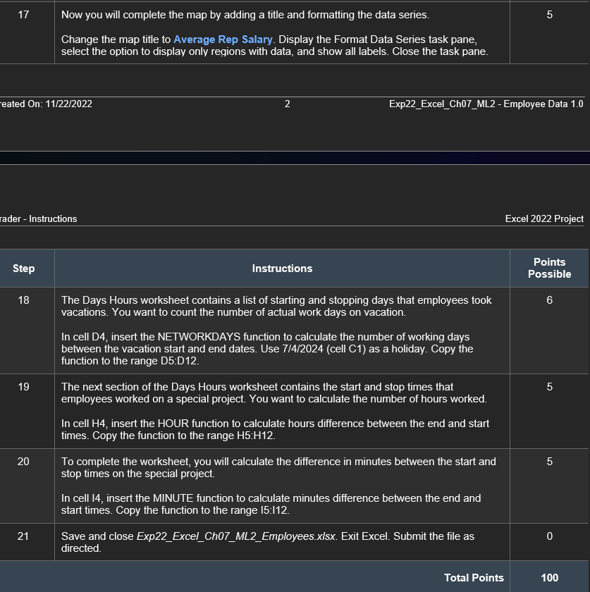\( 17 \quad \) Now you will complete the map by adding a title and formatting the data series. Change the map title to Average Rep Salary. Display the Format Data Series task pane, select the option to display only regions with data, and show all labels. Close the task pane.