Home /
Expert Answers /
Advanced Math /
free-space-green-39-s-function-of-helmholtz-equation-30pts-finding-the-green-39-s-function-g-r-r-39-pa769
(Solved): Free-space Green's function of Helmholtz equation. [30pts]. Finding the Green's function, g(r,r^(')) ...
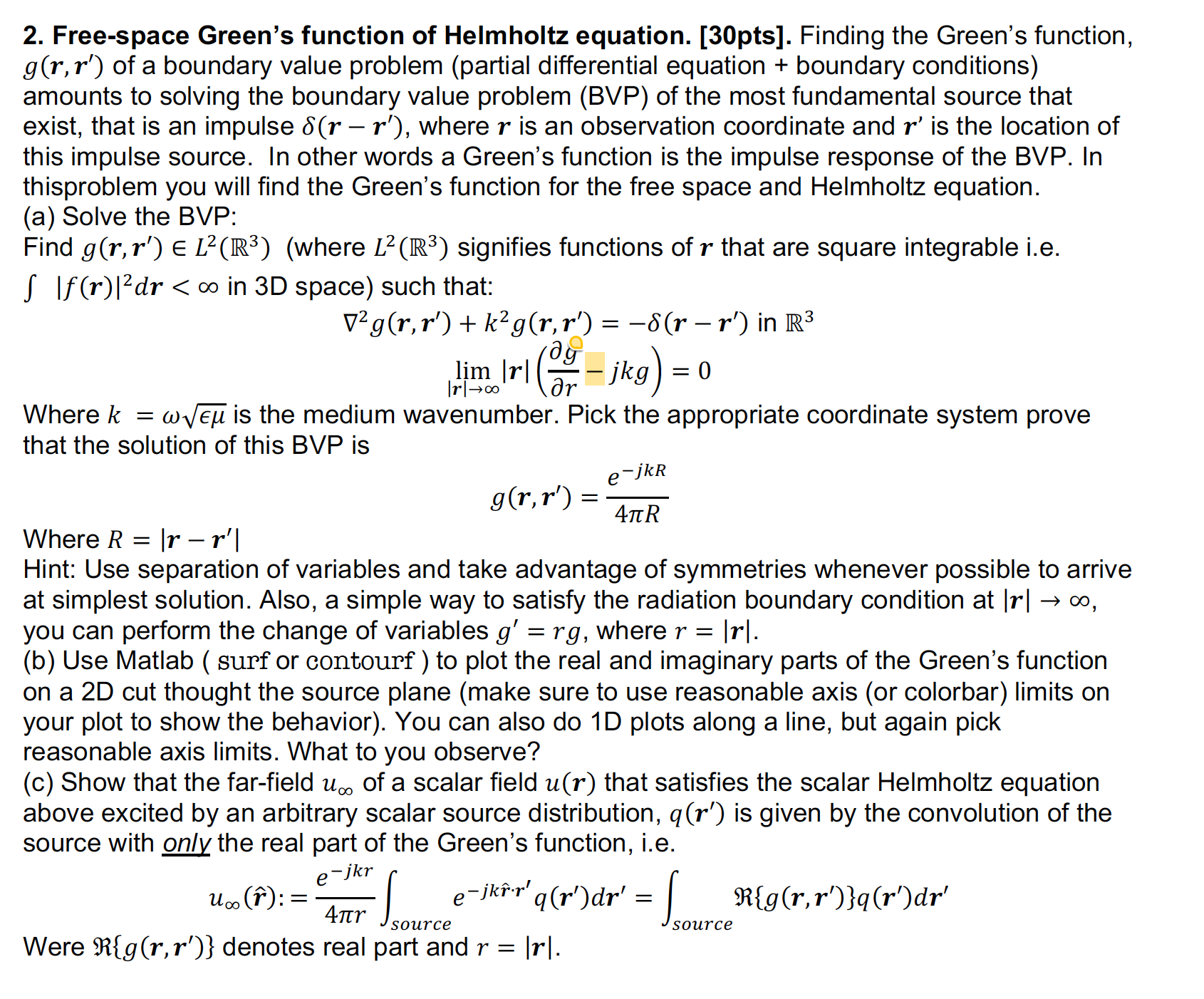
Free-space Green's function of Helmholtz equation. [30pts]. Finding the Green's function,
g(r,r^(')) of a boundary value problem (partial differential equation + boundary conditions)
amounts to solving the boundary value problem (BVP) of the most fundamental source that
exist, that is an impulse \delta (r-r^(')), where r is an observation coordinate and r^(') is the location of
this impulse source. In other words a Green's function is the impulse response of the BVP. In
thisproblem you will find the Green's function for the free space and Helmholtz equation.
(a) Solve the BVP:
Find g(r,r^('))inL^(2)(R^(3))L^(2)(R^(3)) signifies functions of r that are square integrable i.e.
\int |f(r)|^(2)dr<\infty in 3D spacegrad^(2)g(r,r^('))+k^(2)g(r,r^('))=-\delta (r-r^(')) in R^(3)
\lim_(|r|->\infty )|r|((delG)/(delr)+jkg)=0
Where k=\omega \sqrt(\epsi lon\mu ) is the medium wavenumber. Pick the appropriate coordinate system prove
that the solution of this BVP is
g(r,r^('))=(e^(-jkR))/(4\pi R)
Where R=|r-r^(')|
Hint: Use separation of variables and take advantage of symmetries whenever possible to arrive
at simplest solution. Also, a simple way to satisfy the radiation boundary condition at |r|->\infty ,
you can perform the change of variables g^(')=rg, where r=|r|.
(b) Use Matlab ( surf or contourf ) to plot the real and imaginary parts of the Green's function
on a 2D cut thought the source plane (make sure to use reasonable axis (or colorbar) limits on
your plot to show the behavior). You can also do 1D plots along a line, but again pick
reasonable axis limits. What to you observe?
(c) Show that the far-field u_(\infty ) of a scalar field u(r) that satisfies the scalar Helmholtz equation
above excited by an arbitrary scalar source distribution, q(r^(')) is given by the convolution of the
source with only the real part of the Green's function, i.e.
u_(\infty )(hat(r)):=(e^(-jkr))/(4\pi r)\int_(source ) e^(-jkhat(r)r^('))q(r^('))dr^(')=\int_(source ) R{g(r,r^('))}q(r^('))dr^(')
Were R{g(r,r^('))} denotes real part and r=|r|.