Home /
Expert Answers /
Computer Science /
complete-steps-1-16-and-guve-formulas-to-complete-project-to-look-like-final-picture-townsend-mort-pa530
(Solved): Complete Steps 1-16 and guve formulas to complete project to look like final picture. Townsend Mort ...
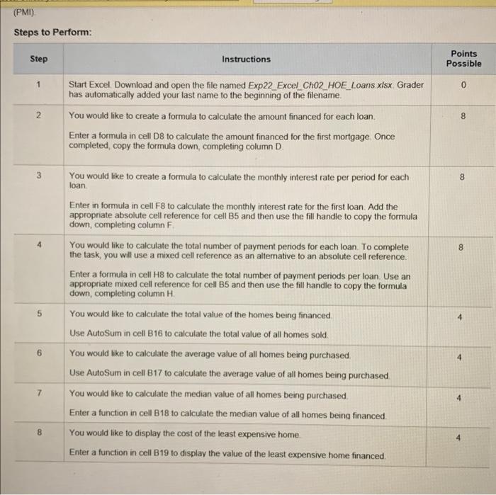
Complete Steps 1-16 and guve formulas to complete project to look like final picture.
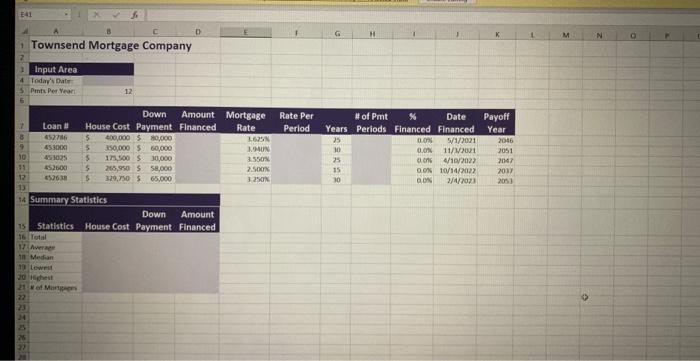
Townsend Mortgage Company
Steps to Perform:
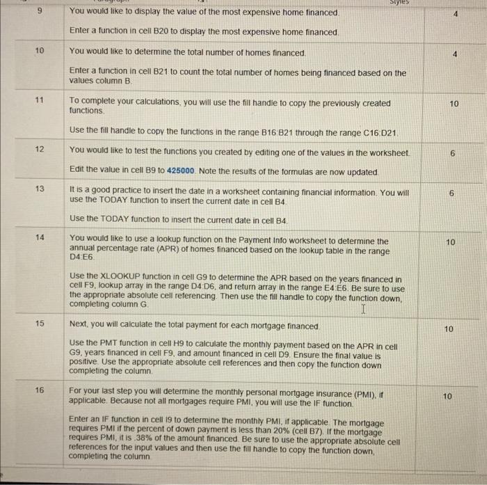
You would like to display the value of the most expensive home financed. 4 Enter a function in cell B20 to display the most expensive home financed. 10 You would like to determine the total number of homes financed. 4 Enter a function in cell B21 to count the total number of homes being financed based on the values column . To complete your calculations, you will use the fill handie to copy the previously created 10 functions. Use the fill handle to copv the functions in the range B16.821 through the range C16.D21. 12 You would like to test the functions you created by editing one of the values in the worksheet. 6 Edit the value in cell B9 to 425000 . Note the results of the formulas are now updated. 13 It is a good practice to insert the date in a worksheet containing financial information. You will 6 use the TODAY function to insert the current date in cell B4. Use the TODAY function to insert the current date in cell B4. You would like to use a lookup function on the Payment Info worksheet to determine the annual percentage rate (APR) of homes financed based on the lookup table in the range D4:E6. Use the XLOOKUP function in cell G9 to determine the APR based on the years financed in cell F9. lookup array in the range D4 D6, and return array in the range E4:E6. Be sure to use the appropriate absolute cell referencing. Then use the fill handle to copy the function down, completing column . 15 Next, you will calculate the total payment for each mortgage financed 10 Use the PMT function in cell H9 to calculate the monthly payment based on the APR in cell G9, years financed in cell F9, and amount financed in cell D9. Ensure the final value is positive. Use the appropriate absolute cell references and then copy the function down completing the column. 16 For your last step you will determine the monthly personal mortgage insurance (PMI), if applicable. Because not all mortgages require PMI, you will use the IF function. Enter an IF function in cell i9 to determine the monthly PMI, if applicable. The mortgage requires PMI if the percent of down payment is less than (cell B7). If the mortgage requires PMI, it is . of the amount financed. Be sure to use the appropriate absolute cell references for the input values and then use the fill handie to copy the function down, completing the column
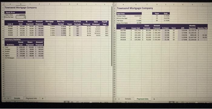
Tewniend Mortgage Company Townsend Mortgage Company
Expert Answer
Step 1: Open the file named "Exp22 Excel_Ch02 HOE_Loans.xlsx"Step 2: Enter a formula in cell D8 to calculate the amount financed for the first mortgag